Welcome to the Newfoundland and Labrador Adaptation Cost-Benefit Analysis (NLACBA) Tool documentation site.

This project was funded by the Government of Newfoundland and Labrador, and carried out by Heron Hydrologic Ltd.

On this page:

1. Introduction
2. Cost-Benefit Analysis Tool
   1. CBA Tool Overview
   2. Repository Organization and Resources
   3. Minimum System Requirements
   4. Installation and Usage
   5. Software Description
   6. CBA Tool Functions
   7. CBA Datasets
   8. Processing and Assumptions
3. Modifying the CBA Tool
   1. Updating the Spatial Data
   2. Updating the Damage Curves
   3. Using other Return Period Flood Data
   4. Adapting the CBA Tool for Other Hazards
   5. Adjusting the NLACBA Tool Code
4. Additional Resources
   1. Video Tutorials
   2. Example Case Studies
5. Troubleshooting
   1. Common Troubleshooting Tips
   2. Contact our Team
   3. Updates to the Tool
6. Glossary

1 Introduction

• basics of the tool and purpose
• climate change context in Newfoundland and Labrador
• purpose of this project and the tool usage
• other likely benefits of the tool (data repository, use of tool in other jurisdictions, etc.)

2 Cost-Benefit Analysis Tool

2.1 CBA Tool Overview

• Spreadsheet-based decision-support tool for evaluating flood adaptation options
• Developed for small municipalities in Newfoundland and Labrador
• Designed for high-level economic comparison of flood mitigation strategies
• Requires user inputs to define:
  • Flood scenarios
  • Infrastructure type
  • Damage assumptions
  • Economic parameters
• Produces outputs including:
  • Estimated total flood damages by return period
  • Statistics on impacted infrastructure
  • Economic metrics comparing adaptation options against the baseline “No Action” scenario
• Outputs total flood damages under the given scenarios for different return period events, statistics on impacted infrastructure, and economic metrics describing the relative benefit of various options against the baseline ‘No Action’ option

2.2 Repository Organization and Resources

The tool is provided openly by the Province of Newfoundland and Labrador and the project funders under the governmental licensing agreement.

2.3 Minimum System Requirements

• Windows 11 Operating System
• 4 GB of RAM
• License for Microsoft Excel
• 1.6 GB of free space locally

2.4 Installation and Usage

• How to download, install
• Spreadsheet based program
• Make selections in Excel sheet
• Contains the CBA Tool, and data editing modes
• Data editing intended to help users prepare raster data that would be required for analysis within the tool

2.4.1 Installation

The tool is setup for use in Windows by default. For use in a MacOS, see the section below on how the setup and installation differs for a mac operating system.

2.4.1.1 Download the Tool

• Access the CBA Tool package from the host server (link provided by your project administrator).
  Click the download link to save the .zip file to your computer.

2.4.1.2 Extract the Files

• Once downloaded, navigate to the .zip file in your file explorer.
• Right-click on the file and select “Extract All…” from the context menu.
• When prompted, choose your preferred directory (e.g., C:\Users\YourName\Documents\CBA_Tool) where the extracted files will be stored.
• Click Extract to unpack the tool into the selected folder.

2.4.1.3 Confirm Installation

• Open the extracted folder and verify that it contains the necessary files (e.g., executable, supporting scripts, and documentation).

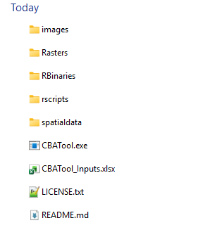
• You are now ready to launch the CBA Tool from the chosen directory.

2.4.1.4 Security and File Permissions

The CBATool_Inputs.xslx is a regular Excel spreadsheet that does not require macros or other security settings to be enabled, so this file should be usable as long Microsoft Office is installed with MS Excel.

The CBATool.exe file is an executable program that may require IT permissions to allow it to run, especially if you are on a managed machine. If you have admin privileges and the executable becomes blocked, you can try these steps.

1. Open Windows Security on your computer.
2. Go to Virus & threat protection tab.
3. Click on the Protection history option.
4. Choose an app that you want to allow (in this case, CBATool.exe).
5. Click on the Yes button in UAC prompt.
6. Click on the Actions button.
7. Choose Allow on device option.
8. Click the Yes button.

Note: if you do see a blue screen that says ‘Windows protected your PC’ when trying to run the tool, you can click on More info and Run anyway.

2.4.1.5 MacOS Installation

For running this tool on a MacOS, a few additional steps are needed. The R installation that comes with the tool is setup for Windows, so a local R installation is needed for a mac or linux operating system.

Follow the steps below to run the tool for MacOS.

1. Install R – visit the website (R for MacOS)[https://cran.rstudio.com/bin/macosx/] and download either the silicone or intel-based .pkg file, depending on the era of your mac machine. You can check this by clicking on the apple icon on the top left corner, About This Mac, and checking if the processor mentions Intel (meaning an Intel processor), else if it says M1 or M2, it is a silicone chip.
2. Double click on the pkg file that was downloaded, and follow instructions to install R. You should have version 4.5 or greater installed.
3. Download and unzip the nlacba zip file from the available website using the same instructions as Windows (finding the folder in the Finder rather than Windows Explorer).
4. From the Launchpad, open the Terminal application.
5. In the Terminal, navigate to the downloaded nlacba folder using the cd command. This may be something like: cd Downloads/nlacba_20230401
6. If you do not have the R package openxlsx installed, you will need to install this as well. This can be done by:
   1. in Terminal, type R
   2. enter the command below and follow the prompts: install.packages(‘openxlsx’)
   3. enter q() and hit n to return to the Terminal
7. Run the tool in Terminal by entering the following command: Rscript.exe ./rscripts/dispatcher.R
8. If you encounter more errors about missing packages, you may need to repeat step 6 to install packages locally, replacing the openxlsx with the name of the missing package.

If you require support on getting the tool to work in a mac or linux environment, please Contact us for support.

2.4.2 How to Use

Open the CBATool_Inputs.xlsx file to begin using the tool.

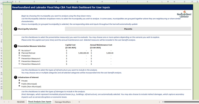
This figure provides an overview of the Newfoundland and Labrador Flood Map CBA Tool main dashboard, showing the available user input options. Users can define key settings such as municipality, preventative measures, infrastructure type, damage types, flood type, and cost multipliers. Dropdown menus, checkboxes, and entry fields are used to customize inputs, with default values automatically assigned where applicable.

2.4.2.1 Step 1 – Select Municipality

Use the drop-down menu to select the municipality of interest.

Municipalities located in close proximity (e.g., Victoria, Carbonear, Salmon Cove) can also be grouped together for combined analysis.

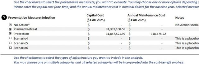
2.4.2.2 Step 2 – Choose Preventative Measures

After selecting the municipality, use the checkboxes to define which preventative measures you would like to include in the analysis.

Preventative Measure Options

• No Action
  Baseline condition with no preventative measures applied.
• Planned Retreat
  Establishes a 100-metre buffer from the coastline, with affected assets assumed to have zero retained value.
• Protection
  Implementation of engineered or structural measures to defend against flooding.
• Stabilization
  Shoreline reinforcement or land stabilization measures to reduce flood risk.
• Abandonment
  Withdrawal from at-risk areas without replacement or protective intervention.
• Accommodation
  Adjustments to buildings or land use (e.g., elevating structures, floodproofing) to reduce vulnerability while continuing occupancy.

2.4.2.3 Step 3 – Select Infrastructure of Interest

Next, use the checkboxes to define the type of infrastructure to include in the analysis. You may select one or multiple options depending on the scope of the assessment.

Infrastructure Options

• Private
  Infrastructure owned and maintained by individuals, businesses, or private organizations (e.g., residential homes, commercial buildings).
• Public
  Infrastructure owned and maintained by government authorities (e.g., schools, hospitals, municipal buildings, emergency services).
• Public Non-Municipal
  Infrastructure owned and operated by non-municipal public entities, such as provincial or federal agencies (e.g., highways, utilities, and regional facilities).

2.4.2.4 Step 4 – Select Damages to Include

After defining the infrastructure of interest, use the checkboxes to choose the type of damages to include in the analysis. Users may select either or both options depending on the scenario being evaluated.

Damage Options

• Direct Damages
  Immediate physical or structural damages to infrastructure and assets caused by flooding (e.g., building repairs, replacement costs).
• Indirect Damages
  Secondary or consequential impacts that occur as a result of flooding (e.g., business interruption, loss of services, or increased transportation costs).

2.4.2.5 Step 5 – Define Cost Multiplier

The next step is to specify the cost multiplier that will be applied to calculate damages. By default, the tool automatically assigns a general cost multiplier based on the selected municipality. This default value ensures that regional cost factors are accounted for in the analysis.

If users would prefer to apply their own adjustment, they can override the default value. To do this, simply enter the desired multiplier in the bolded box labeled Override cost multiplier. This allows for customization if local data, expert knowledge, or project-specific conditions suggest that the general cost multiplier is not appropriate. All cost multipliers are referenced from pricing in St. John’s.

2.4.2.6 Step 6 – Select Flood Type

Next, use the drop-down menu to select the flood type for the analysis. The available options are:

Flood Type Options

• Coastal
  Considers damages and preventative measures related only to coastal flooding.
• Coastal and Riverine
  Considers combined flooding impacts from both coastal and riverine (inland river system) sources.

If the Coastal and Riverine option is selected but a river system is not available for the chosen municipality, the tool will display the following message:

WARNING: Riverine data not available for selected municipality

In this case, the analysis cannot proceed. Users will need to either select Coastal instead, or provide the Coastal & Riverine depth rasters manually before re-running the tool. This can be done by importing the .tif rasters in the following directory: /Rasters/Municipality_Name. Note that Municipality_Name represents the municipality the user chose while filling out the CBATool_Inputs.xlsx file

2.4.2.7 Step 7 – Select and Run Tool

Once the primary settings have been defined, users can choose which tool they would like to run. Five options are available:

Tool Options

• Run CBA Tool
  Executes the full cost–benefit analysis based on the selected municipality, preventative measures, infrastructure of interest, damages, flood type, and cost multiplier. This is the standard option for generating outputs and results.
• Raster Editor
  Opens a raster editor where users can modify depth rasters through a built-in editor, applying effects such as setting or multiplying depth values within a user-defined polygon area. The edited raster can then be saved for a specific preventative measure and used in subsequent calculations.
• Spatial Data Viewer
  Provides a spatial viewer for exploring the vector layers used in the tool, such as buildings, roads, and other infrastructure. This mode is useful for reviewing input data, validating coverage, and understanding the spatial context before running the analysis. Suggestions for changes to the data can be requested for specific IDs shown in the viewer.
• Create Study Boundary Tool
  Opens an interactive map interface that allows users to define a custom study area for analysis. Users can draw, edit, and refine a polygon boundary to limit the assessment to a specific neighborhood, infrastructure corridor, or area of interest within a municipality. Saved study boundaries are automatically detected by the CBA Tool, and when present, all exposure, damage, and economic calculations are restricted to the defined boundary extent.
• Measure Tool
  Opens an interactive map interface that allows users to directly measure the lengths and/or areas of potential protection measures, and also estimate the height that would be required of the structure. The Measure Tool can be used in conjunction with the Cost Estimator to estimate the cost of different protection measures.

2.4.2.8 Step 8 – Define Menu Type

Finally, users can define the menu type using the drop-down menu. Two options are available:

Menu Type Options

• Basic
  Runs the tool using the default settings defined within the template. This option is sufficient for most general applications and requires minimal customization.
• Advanced
  Allows users to overwrite key input parameter values, providing greater flexibility and control. Advanced options include:
  • Social Discount Rate (%) – Used to adjust the present value of future damages and benefits.
  • Design Time (years) – The time horizon for the analysis.
  • Vehicle Minimum Depth (m) – The water depth at which vehicle damages begin to occur.
  • Vehicle Maximum Depth (m) – The water depth at which total vehicle damages are assumed.
  • Average Vehicle Cost – The representative value of vehicles considered in the analysis.

In addition, users can select which direct damage layers to include (e.g., buildings, roads, airports) and which indirect damages to apply, such as:

• Emergency Damage Ratio (%) – Represents the proportion of emergency-related losses.
• Economic Damage Ratio (%) – Represents the proportion of broader economic losses.

2.4.3 Step 9 – Run the Executable

Once all input variables have been defined, save your changes to the spreadsheet (Ctrl+S) and navigate to the tool folder on your computer.

Double-click on CBATool.exe to launch the program. A command window will appear — allow it to run uninterrupted until it closes automatically. Do not manually close this window.

When the window closes, return to the tool folder. A new folder named outputs will have been generated. This folder contains the results of the analysis and can be used for further review and reporting.

2.5 Software Description

• R-based processing – The tool runs on R scripts to handle data and analyses.
• Self-contained package – All required scripts, binaries, and libraries are bundled with the tool.
• No external dependencies – It does not require or use any existing R installation on your system.

This tool uses R scripts behind the scenes to process data and perform analyses. All scripts are stored in the rscripts folder and are compiled and executed through the CBATool.exe application. The R binaries are packaged and included with the tool to ensure portability, so no separate R installation is required. The tool relies on its own local R library within the tool folder and will not use or depend on any existing R installation on your system.

2.6 CBA Tool Functions

2.6.1 Raster Editor Tool

The Raster Editor is a tool within the CBA architecture that provides users with a simple and flexible interface for modifying the coastal flood depth rasters. This functionality is intended to help users adjust and visualize potential infrastructure or adaptation measures that are not yet represented in the existing geospatial datasets. For example, newly constructed seawalls, raised coastal roads, or other protective infrastructure implemented by municipalities can be easily compared to a no action scenario.

Purpose and Functionality

In many cases, baseline coastal depth rasters represent “current conditions”. They do not reflect proposed or hypothetical flood mitigation measures. The Raster Editor allows users to edit or adjust these rasters to simulate the effects of such interventions. This allows stakeholders to estimate how various coastal protection strategies could change flood extents, depths, and resulting damages.

Specifically, the Raster Editor allows users to:

• Modify raster cell depth values directly to simulate new or modified land elevations (e.g., seawall construction, land raising, dike improvements)
• Apply uniform depth adjustments (add, subtract, or replace values) within user-defined polygon areas.
• Define buffer zones around infrastructure or coastal features and assign adjusted “set depth” values.
• Save edited rasters under unique scenario names for later use in the CBA Tool’s damage and economic calculations.

How It Works and How to Find Saved Datasets

When the Raster Editor mode is launched from the CBA Tool (Step 7 – Select and Run Tool), users are presented with a map-based editing interface. From here, the process typically follows these steps:

• Load Raster: Select the municipality or raster dataset you wish to edit. The associated coastal depth raster will be displayed. This is done in the CBATool_Inputs.xlsx excel sheet before the application is executed. When the Interactive Raster Editor window pops up, select and/or confirm the municipality, scenario, prevention measure, and flood type. When all is confirmed, click the Load Raster button and then the Zoom to Raster Extent button.
• Edit Raster: Draw or import a polygon representing the area of modification. This could represent a new seawall alignment, elevated coastal road, or other infrastructure zone. Apply cell numerical modifications to reflect these changes.
• Under the Edit Raster Tab, users can choose the desired edit type:
  • Edit Mode: Set – Replace all raster cells within a drawn polygon with a specified depth value. Done by selecting the “set” button.
  • Edit Mode: Add/Subtract – Modify existing raster values by a specified amount.
  • Edit Mode: Multiply – Modify existing raster values within a polygon area by multiplying them by a coefficient.
  • Apply Edit Outside Selected Area – A dedicated option enables the user to apply the chosen raster edit outside the selected polygon instead of inside it. This allows for inverse edits. This is useful when the selected area should remain unchanged while the surrounding area is modified.
  • Prevent negative values – Options to convert negative values to null values or zero
  • Buffer Adjustment – Create a buffer around a selected feature and assign a new spatially edited depth or adjusted value
• Apply and Preview Changes: The tool recalculates and displays the modified raster section, allowing users to visually confirm the intended changes before saving
• Save the Edited Raster: Once edits are finalized, the modified raster can be saved as a new file under the Save Raster tab. The tool assigns a unique scenario name (e.g., 20yr_Planned Retreat_edited.tif). Saved rasters are stored in the /Rasters/Municipality_Name sub-folder within the tool’s working directory. Note that Municipality_Name represents the municipality the user chose while filling out the CBATool_Inputs.xlsx file. The directory to the saved raster is displayed when the Save Raster button is clicked. Rasters must have _edited appended at the end of their names to be utilized in the tool.
• Use in Analysis: Edited rasters can then be referenced in the CBA Tool under the selected municipality and flood type. When running the analysis, the tool will use the adjusted raster values to recalculate flood damages and economic metrics for that scenario.

Example Usage

A municipality planning a new seawall could:

• Open the Raster Editor and load the coastal flood raster for the town.
• Apply a 50 m inland buffer around the seawall by drawing a polygon around the buffer area and set the depth value within the buffer to zero (to simulate full protection).
• Save the edited raster using the Save Raster button.
• Re-run the CBA Tool using the saved raster to estimate reduced flood damages and the resulting benefit-cost ratio compared to the baseline “No Action” case. Note that the Raster Editor tool creates a file that appends _edited to the original file name. If that new raster file (with _edited in its name) is found when running the tool, it is picked up and used automatically instead of the unedited raster. Therefore, no manual moving or renaming of files is needed.

Notes and Best Practices

• Edited rasters are intended for exploratory and planning-level analysis only. They are not substitutes for detailed hydraulic or coastal modeling.
• Users should document all raster edits, including the assumptions used for buffer widths, elevation changes, and protective structures.
• For reproducibility, consider maintaining a log file of each raster edit scenario with details on edit date, applied depth or spatially edited depth values, and reasoning.
• If unsure about reasonable depth adjustments, consult with a qualified coastal engineer or flood risk specialist.

2.6.2 Spatial Data Viewer Tool

The Spatial Data Viewer Tool provides users with an interactive, web-based interface for viewing, exploring, and editing spatial datasets used in the Cost-Benefit Analysis (CBA) Tool. It was designed to make it easier for municipalities, planners, and other stakeholders to understand the spatial context of the analysis and to contribute improved or corrected geospatial information when more accurate local data is available.

This tool serves as a quality assurance and collaboration feature, enabling users to visually inspect datasets such as buildings, land use, and infrastructure, and to provide data updates that improve the accuracy of future analyses.

Purpose and Functionality

The Spatial Data Viewer allows users to:

• View all CBA datasets (e.g., buildings, roads, airports etc…) in an interactive map viewer directly within their web browser.
• Explore and query dataset attributes by selecting individual features on the map.
• Identify and correct data inaccuracies — for example, if a feature’s classification or land-use type is incorrect.
• Suggest edits to datasets by referencing the feature’s unique ID and submitting updated attribute information to ECCInfo@gov.nl.ca.
• Save revised or improved spatial layers for re-use in subsequent analyses.

This tool ensures that the CBA results reflect the most accurate and locally verified data possible.

How It Works and How to Find Datasets

When the Spatial Data Viewer Tool is launched (from Step 7 – Select and Run Tool), a browser window opens displaying an interactive map with all CBA spatial datasets loaded. Users can toggle layers on or off, click features to view attributes, and make note of any corrections.

The typical workflow is as follows:

• Load Map and Datasets: The viewer automatically displays all relevant spatial datasets for the selected municipality, including building footprints, land use, infrastructure, and flood layers.
• Inspect Features: Click on individual features to display their attributes and metadata.
• Propose Edits: If an attribute is incorrect (e.g., a building categorized as Residential (Detached) should actually be Residential (Apartments) or the ownership of a building polygon should be public (municipal) and not private), the user can record the feature’s ID and submit the corrected information to ECCInfo@gov.nl.ca for review.
• Save Updated Layers: Once edits have been validated, users can export or save a revised geospatial layer.
• Re-run the CBA Tool with Updated Data: To re-run the tool using an updated dataset, replace the corresponding file in the appropriate folder. For example, an updated building dataset should be saved as: /spatialdata/NL_Buildings/NL_buildings.gpkg

Replace the existing file with the new version and re-run the tool to apply the updated data to the analysis.

All datasets can be found in the spatialdata directory within the CBA Tool’s main working folder.

Example Usage

A municipality notices that several buildings in its jurisdiction are misclassified as Residential (Detached) when they are actually Residential (Apartments). The workflow would be:

• Launch the Spatial Data Viewer Tool to display the local datasets.
• Select the misclassified buildings and note their feature IDs.
• Provide corrected classifications and send the updated information to ECCInfo@gov.nl.ca.
• Once approved, update the building dataset (NL_buildings.gpkg) under /spatialdata/NL_Buildings/NL_buildings.gpkg.
• Re-run the CBA Tool with the updated dataset to generate new results that reflect the corrected land-use data.

Notes and Best Practices

• Always reference the feature ID when suggesting or applying edits to ensure consistency between datasets (not the feature fid).
• Maintain a record of all suggested or applied edits, including date, feature ID, and rationale.
• When submitting updates to ECCInfo@gov.nl.ca, include both the revised dataset and a short summary of changes.
• Verify that replacement datasets maintain the same coordinate reference system (CRS) and attribute schema as the original file.
• Use the viewer primarily for data review and light attribute correction – it is not intended for complex spatial analysis or heavy geoprocessing.
• For transparency and reproducibility, save each updated dataset with a descriptive name and document all modifications before replacing existing files.

2.6.3 Create Study Boundary Tool

The Create Study Boundary Tool enables municipalities to draw, edit, and save a custom geographic boundary that defines the extent of the area to be analyzed in the Cost-Benefit Analysis (CBA) Tool. This functionality is essential when municipalities need to limit the analysis to a specific neighborhood, infrastructure corridor, flood-prone zone, planning district, or other area of interest within the municipality area. This tool improves the relevance, precision, and efficiency of the CBA, ensuring that the results reflect the geographic extent most meaningful for local decision-making.

Purpose and Functionality

The Create Study Boundary Tool allows users to:

• Draw a Custom Boundary directly within an interactive map interface using tools such as polygon drawing, editing, moving, and deleting vertices.
• Edit an Existing Boundary by adjusting vertices or reshaping its extent.
• Save the Final Boundary to a standardized location so that it can be used directly by the CBA Tool.
• Run the CBA Using the Defined Boundary, ensuring only the selected geographic area is included in exposure, damage, and cost-benefit calculations.
• Add a custom study boundary created from another GIS program that is saved as a geopackage file under /spatialdata/study_boundary.gpkg.

This tool helps municipalities tailor their analyses to local planning priorities and encourages consistency across repeated analyses.

How It Works and How to Find Datasets

When the Create Study Boundary Tool is launched (from Step 7 – Select and Run Tool), a browser window opens displaying a base map of the municipality. The user can then create or import a boundary and save it for use in the CBA.

The typical workflow is as follows:

1. Initialize Map: The map displays the municipal extent along with relevant reference layers (e.g., roads, buildings, coastlines) to guide accurate boundary drawing.
2. Create or Import Boundary
   1. Zoom to Municipal Bounds: Zoom the map to the municipality of interest
   2. Load Existing Boundary: Load a boundary already created previously (Geopackage .gpkg format)
   3. Draw Boundary: Use interactive drawing tools to sketch a polygon around the desired study area.
   4. Save Study Boundary: Save the study boundary created in the map interface to a file within the tool
3. Edit Boundary Geometry: Users can refine the boundary by moving vertices, deleting points, or redrawing portions until the desired extent is captured.
4. Save Boundary File: The finalized boundary is saved in the CBA Tool’s working directory under: /spatialdata/study_boundary.gpkg
5. Run the CBA with the Boundary: When the CBA Tool is executed, it automatically checks for the presence of study_boundary.gpkg. If found, all subsequent analysis steps (exposure, damages, costs, avoided losses, and benefit-cost ratio) are performed only within the defined boundary.

Example Usage

A municipality wants to evaluate the economic benefits of flood protection measures for a specific downtown district rather than the entire city.

Steps:

1. Launch the Create Study Boundary Tool.
2. Draw a polygon around the downtown area using the map interface.
3. Adjust the geometry until it matches the district boundary.
4. Save the file as study_boundary.gpkg in the designated directory by clicking the Save Study Boundary button.
5. Run the CBA Tool. The analysis will now be limited to the downtown study boundary.

Notes and Best Practices

• Use clear, well-defined boundaries. Avoid small gaps or overlaps, and ensure the polygon fully encloses the target area.
• Maintain consistent Coordinate Reference System (CRS). The saved boundary must match the CRS used by the CBA datasets (EPSG:4326). The tool automatically assigns this CRS to the newly saved boundary file.
• The study area boundary is stored under ./spatialdata/study_boundary.gpkg. If you wish to delete the study boundary, you may remove this file. If you are having issues, please check that this file exists
• If you create your own file outside of the CBA tool, keep naming conventions consistent. The CBA expects the boundary to be saved as ./spatialdata/study_boundary.gpkg with this exact name and folder location
• Document the boundary creation process, including rationale, source data, and date of creation.
• Use the tool for study area definition only. It is not intended for complex digitization tasks or advanced geoprocessing.

2.6.4 Damage Modifiers

Damage Modifiers can be applied to adjust damages at a specific selection of infrastructure based on the Preventative Measure, Class, and ID. The Damage Modifiers can be adjusted in the CBA_Inputs.xlsx file under the Damage Modifiers sheet.

The Damage Modifiers may be most helpful in adjusting the costs for coastal infrastructure, as the damages to coastal infrastructure are not impacted by the depth rasters themselves, but are computed from the data in the Coastal Conditions sheet of the input xlsx file. For breakwater structures, the local conditions and the type of breakwater impact the degree of reduction substantally. However, some general rules of thumb: a large emergent (above the surface of the water) breakwater will provide more relief from storm surges than a submerged. An emergent breakwater may reduce significant wave height up to 90%, while a submerged breakwater may be reduction as low as 20%. The distance of the structure from the shore also controls how much impact the reduction has, and where that reduction may be felt. These numbers may be used to roughly guide the application of Damage Modifiers in the tool and editing in the Raster Editor.

Example Usage

A municipality might use Damage Modifiers to reduce damage at a breakwater structure in a protection scenario.

Steps:

1. Open CBA_Inputs.xlsx file.
2. Launch the Spatial Data Viewer Tool.
3. Locate the desired structure and copy the structure ID.
   
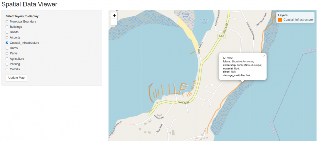
   This figure shows an example of a coastal structure with the ID that will be needed to edit a Damage Modifier.
4. Return to CBA_Inputs.xlsx file.
5. Select the Damage Modifiers sheet at the bottom of the file.
6. Enter the Preventative Measure, Class, ID, and Damage Multiplier.
   
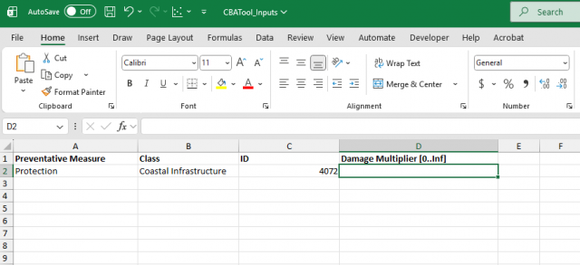
   This figure shows an example of applying a Damage Modifier.
7. Run the CBA Tool. Now the analysis will account for the applied Damage Modifier(s).

2.6.5 Measure Tool and Protection Sheet

Measure Tool

The purpose of this tool is to provide away for users of the NLACBA tool to directly measure the lengths and/or areas of potential protection measures, and also to estimate the height that would be required of the structure. For example, a community considering a seawall could estimate the required length and height of the seawall using this tool.

The Measure Tool is launched by setting the Select Tool in CBATool_Inputs.xlsx to Measure Tool. This opens a window in the default browser, where users can interactively work with the tool.

In the Input tab of the Measure Tool in the left pane of the screen, users can select a municipality, a flood scenario, a flood type, the freeboard (0.3 meters by default), as well as the type of infrastructure.

The freeboard is a factor of safety added above the base flood depth. For example, if the expected/estimated flood depth for a protection wall is 3m, the freeboard is the added extra height. With the default freeboard of 0.3m, the structure would have a height of 3.3m.

Once the inputs are set, click the “Load Raster” button to display the raster on the map.

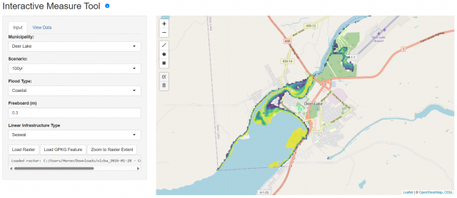
This figure shows the Interactive Measure Tool launched in the browser with the inputs pane on the left side and the interactive map on the right side.

Within the interactive map section, users can select “Draw a polyline” or “Draw a polygon”:

• Selecting “Draw a polyline” allows the user to draw a line on the map capturing the desired length and depth of the proposed infrastructure. Once a polyline is drawn, select the View Data tab to view the results.
• Selecting “Draw a polygon” allows the user to draw a polygon on the map capturing the desired area of the proposed infrastructure. Once the polygon is drawn, select the View Data tab to view the area of the polygon.

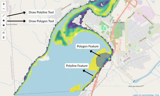
This figure shows the polyline and polygon features drawn by the user.

As the features are added, the View Data tab displays the length of the polyline and the corresponding average depth for polylines, and a different table will show for polygon areas. The table can be downloaded as a .csv (Excel) file. The drawn features can be downloaded as a geopackage (.gpkg) file. In addition, these geopackage files can be loaded into the map using the Load GPKG Feature button in the Input tab.

Depth_m represents the depth in meters of the feature without the freeboard , while Depth_fb_m represents the depth in meters with the freeboard.

The Building Areas button in the View Data tab shows the total area of the buildings within the drawn polygon. This serves as a tool to estimate the planned retreat cost.

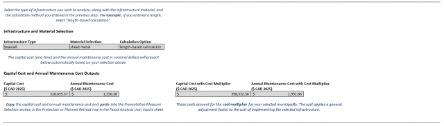
Protection Sheet

The purpose of the sheet is intended to have users input the length, area, or volume of a protection measure that they are considering, and allow the user to estimate the cost of the protection measure as an upfront capital and annual maintenance cost. These estimates can then be populated into the main cost input of the CBA tool.

This sheet is intended to work in conjunction with the Measure Tool, which estimates the length and/or area, as well as the required height of structures, and these values are then exported and entered into the protection sheet for estimating costs.

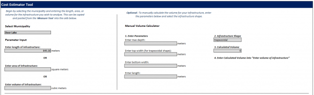
This figure shows the main screen where the user can enter the desired inputs.

The user can input the desired infrastructure type, material of infrastructure, and the calculation option based on the inputted length/area. The tool will automatically estimate the cost of implementing the protection measure.

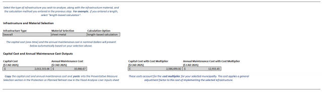
For example, if the user would like to calculate the cost of implement a 100m sheet metal seawall, the procedure would be:

1. Enter 100m into the “Enter length of infrastructure” box. Simply enter “100” because the units in meters are already accounted for
2. Go to the right side of the page and under Linear Infrastructure select “Seawall” from the Infrastructure Type drop down list
3. Select “sheet metal” from the Material Selection drop down list
4. Select “length-based calculation” from the Calculation Option drop down list because 100m was entered as the length. If a area was entered, the user should select “area-based calculation”
5. The total cost will automatically calculate in the Total Cost box

This figure shows 100m inputted as the length of the sheet metal seawall and displays the total cost of a 100m sheet metal seawall.

These cost estimates can then be inserted as a capital cost and annual maintenance cost into the CBATool_Inputs.xlsx file in the main directory, in the section for the costs of each preventative measure.

This figure shows the Capital Cost and Annual Maintenance Cost columns where the calculated costs can be inputted from the Protection Sheet.

2.7 CBA Datasets

This section summarizes the data sources, processing steps, and spatial workflows used to generate each of the infrastructure datasets included in the Cost-Benefit Analysis (CBA) Tool. For each dataset (otherwise known as a geospatial layer), relevant open data sources were compiled, reviewed against satellite imagery, and standardized to ensure consistent categorization across the province.

Each layer includes the following standardized attributes utilized for classification and damage calculation. Every dataset (geospatial layer) provided must contain these attribute fields for the CBA tool to run and produce outputs. All geospatial merging & processing was done in QGIS.

 

Field name	Description
ID	Unique identifier for internal CBA tool processing
fid	Unique identifier created by QGIS for .gpkg files
municipality	Municipality where feature is located in
region	Region where feature is located in
fclass	General classification of feature
area_m2 or length_m	Footprint area if layer consists of polygons. Length if layer consists of lines
ownership	Classification of feature ownership as Private, Public (Municipal), or Public (Non-Municipal)

Agriculture

Data sources & compilation

The agriculture layer in the Cost-Benefit Analysis (CBA) Tool was created using agricultural land use features sourced from the OpenStreetMap (OSM) database. These features were retrieved using the QuickOSM plugin in QGIS and include polygons tagged as farmland, pastures, orchards, vineyards, and other agricultural uses. In addition, the Government of Canada 2020 Land Cover of Canada dataset was consulted to verify agricultural classifications and identify broader agricultural regions not fully captured in OSM. All features were visually reviewed against Google’s satellite imagery to verify positional accuracy and identify areas where OSM coverage may be limited.

Merging & processing

Once collected, the agriculture features were converted to GeoPackage (*.gpkg) format and reprojected to EPSG:3857. Geometry issues were corrected using the “Fix Geometry” tool, and redundant attributes were removed to streamline processing within the CBA Tool.

Additional attributes

None. Only the standardized attribute fields are included.

Classification and ownership list

It must be noted that ownership categorization can be subject to change. However, the general consensus on ownership for each classification is outlined below. Attribute data was standardized to simplify downstream processing within the CBA Tool. Raw agriculture type information from QuickOSM was considered and coded into a consistent classification system.

fclass	ownership
farmland	Private
farmyard	Private
greenhouse_horticulture	Private
meadow	Private

Update potential

Since this agriculture layer is derived from open data sources, it can be updated as more accurate data or improved airport classification information becomes available. If you notice an agriculture layer polygon that appears to be incorrectly classified or that any of the attribute fields do not contain the correct data, you can submit a manual update suggestion through the Spatial Data Viewer tool. Simply copy the agriculture polygon ID (not fid) and send it to ECCInfo@gov.nl.ca, along with the recommended agriculture fclass or ownership correction.

Airports

Data sources & compilation

The airport layer in the Cost-Benefit Analysis (CBA) Tool was created primarily using airport and airfield features sourced from the OpenStreetMap (OSM) database. Additional airport locations and facility information were consulted from the Government of Newfoundland and Labrador’s Airport Services reference website (https://www.gov.nl.ca/ti/airportservices/) to ensure provincial coverage and verify operational sites. All airport locations were overlaid on Google Satellite imagery within QGIS to confirm spatial accuracy and detect airports not captured by the initial datasets. To assist with this process, an image scrapper was applied to identify and flag candidate airport areas based on visual patterns and runway-like infrastructure. The flagged airports were then reviewed, manually polygonized, and integrated into the airport dataset.

Merging & processing

After collection, all airport features were converted to GeoPackage (*.gpkg) format and reprojected to EPSG:3857. Geometry was corrected using the “Fix Geometry” tool, and duplicate features were removed where overlapping or inconsistently attributed. Redundant or non-essential fields were standardized or removed to improve compatibility within the CBA Tool.

Additional attributes

None. Only the standardized attribute fields are included.

Classification and ownership list

It must be noted that ownership categorization can be subject to change. However, the general consensus on ownership for each classification is outlined below. Attribute data was standardized to simplify downstream processing within the CBA Tool. Raw airport type information from QuickOSM was considered and coded into a consistent classification system.

fclass	ownership
airport_regional	Depends but generally Public (Non-Municipal)
apron	Depends but generally Public (Non-Municipal)
runway	Depends but generally Public (Non-Municipal)

Update potential

Since this airport layer is derived from open data sources, it can be updated as more accurate data or improved airport classification information becomes available. If you notice an airport that appears to be incorrectly classified or that any of the attribute fields do not contain the correct data, you can submit a manual update suggestion through the Spatial Data Viewer tool. Simply copy the airport polygon ID (not fid) and send it to ECCInfo@gov.nl.ca, along with the recommended airport fclass or ownership correction.

Buildings

Data sources & compilation

The building layer in the Cost-Benefit Analysis (CBA) Tool was created by compiling a total of three building footprint datasets, including:

• Open Building Population Layer (OBPL) sources automatically extracted from Microsoft’s Bing Mapping system, (https://maximfortin.com/project/obpl-ca-2021/)
  NRCan’s automatically extracted building dataset, (https://open.canada.ca/data/en/dataset/7a5cda52-c7df-427f-9ced-26f19a8a64d6) and
  OpenStreetMap building sources retrieved directly through the QuickOSM plugin in QGIS (https://docs.3liz.org/QuickOSM/)

Once collected, all the datasets were imported into QGIS, and quality assurance and control was performed against Google’s satellite imagery to ensure building positions were well aligned and that areas lacking coverage were identified. NRCan footprints demonstrated the highest positioning accuracy and were therefore considered the base reference map during the merging process.

Merging & processing

QuickOSM and OBPL datasets were merged in a disjoint manner to avoid duplication of data in overlapping polygons. Before merging, all datasets were converted to GeoPackage (*.gpkg) format, and all layers were referenced using EPSG:3857. During this stage, layers were processed using the “Fix Geometry,” “Reproject Layer,” and “Extract by Location” tools in QGIS.

The resulting merged product consists of approximately 338,000 building polygons, each representing a distinct building footprint. This comprehensive layer provides full coverage of Newfoundland and Labrador and serves as a critical spatial data component used by the CBA Tool to estimate direct flood damages to buildings.

Additional attributes

The property and land values filled in this dataset were generated using a regression model. This model uses known land and property values from the MAA data to learn how characteristics such as building area, building type, owernship, and municipality influence value. These relationships are then applied to estimate values for buildings where this information is missing or unavailable. The resulting estimates are joined back to the building footprints so they can be mapped and used directly in GIS analyses.

Field name	Description	Example
institution_class	More specific classification from QuickOSM query	water_works
PROPERTY.VALUE	Property value collected from MAA	134500
LAND.VALUE	Land value collected from MAA	58255.95
PROPERTY.VALUE_filled	Regression model used to estimate missing property values from MAA	67255.55
LAND.VALUE_filled	Regression model used to estimate missing land values from MAA	144500

Classification and ownership list

It must be noted that ownership categorization can be subject to change. However, the general consensus on ownership for each classification is outlined below. Attribute data was standardized to simplify downstream processing within the CBA Tool. Raw building type information from QuickOSM was considered and coded into a consistent classification system, including residential, commercial, industrial, and public categories. Buildings lacking building type attributes were treated with inferred general building types based on their polygon area sizes.

fclass	ownership
Commercial	Private
Fire Station	Public (Municipal)
Gas Station	Private
Hospital	Public (Non-Municipal)
Industrial	Private
Institutional & Government	Public (Non-Municipal)
Public & Civic Infrastructure	Public (Municipal)
Recreation & Leisure	Public (Municipal)
Religious Institution	Private
Residential (appartments)	Private
Residential (cabin)	Private
Residential (detached)	Private
Residential (dormitory)	Public (Non-Municipal)
Residential (general)	Private
Residential (house)	Private
Residential (semidetached)	Private
Residential (static_caravan)	Private
Storage	Private
Temporary & Informal Structures	Private
Transportation & Utilities	Public (Non-Municipal)
Under Construction / Miscellaneous	Private

Update potential

Since this building layer is derived from open data sources, it can be updated as more accurate data or improved building classification information becomes available. If you notice a building that appears incorrectly classified, you can submit a manual update suggestion through the Spatial Data Viewer tool. Simply copy the building ID and send it to ECCInfo@gov.nl.ca, along with the recommended building fclass or ownership correction.

Coastal Infrastructure

Data sources & compilation

The coastal infrastructure layer in the Cost-Benefit Analysis (CBA) Tool was compiled from multiple authoritative and open-data sources to ensure completeness and spatial accuracy across Newfoundland and Labrador. Primary feature locations – including seawalls, breakwaters, and shore protection structures, were extracted from the OpenStreetMap (OSM) database. Additional verified coastal infrastructure datasets and reference material provided through Government of Newfoundland and Labrador resources were incorporated to supplement OSM and ensure provincial coverage.

To capture unmapped coastal structures, aerial and satellite imagery (Google Satellite) was reviewed in QGIS. An image scraper was applied to automatically identify and flag potential missing infrastructure locations based on visual shoreline patterns and structural characteristics (e.g., dock geometry, linear coastal armouring). All flagged features were reviewed by hand, and missing infrastructure was manually digitized and classified as line or polygon features, depending on structure type.

Merging & processing

Once collected, all coastal infrastructure features were standardized into a common GeoPackage (*.gpkg) format and reprojected to EPSG:3857 for consistency with other CBA spatial layers. Geometry integrity was validated using the Fix Geometry tool, and redundant or overlapping attributes were consolidated. Duplicate features were removed, and attribute fields were standardized to ensure alignment with CBA Tool schema conventions, including fields for structure type, ownership class, and municipal context.

Additional attributes

Field name	Description	Example
slope	slope value (in degrees)	90
damage_multiplier	–
material	construction material of infrastructure	Stone
bathyelev	–	2.09
offshoreelev	–	-7.70
shielding_ID	–	NA

Classification and ownership list

It must be noted that ownership categorization can be subject to change. However, the general consensus on ownership for each classification is outlined below. Attribute data was standardized to simplify downstream processing within the CBA Tool. Raw building type information from QuickOSM and the coastal infrastructure layer from government of newfondland and labrador was considered and coded into a consistent classification system.

Field name	Description	Example
slope	slope value (in degrees)	90
damage_multiplier	–
material	construction material of infrastructure	Stone
bathyelev	–	2.09
offshoreelev	–	-7.70
shielding_ID	–	NA

Classification and ownership list

It must be noted that ownership categorization can be subject to change. However, the general consensus on ownership for each classification is outlined below. Attribute data was standardized to simplify downstream processing within the CBA Tool. Raw building type information from QuickOSM and the coastal infrastructure layer from government of newfondland and labrador was considered and coded into a consistent classification system.

fclass	ownership
Breakwater	Public (Non-Municipal)
Dock	Public (Municipal)
Jetty	Public (Non-Municipal)
Revetment	Public (Non-Municipal)
Seawall	Public (Non-Municipal)
Shoreline Armouring	Public (Non-Municipal)

Update potential

Since this coastal marine infrastructure layer is derived from open data sources, it can be updated as more accurate data or improved coastal marine infrastructure classification information becomes available. If you notice infrastructure that appears incorrectly classified, you can submit a manual update suggestion through the Spatial Data Viewer tool. Simply copy the infrastructure ID and send it to ECCInfo@gov.nl.ca, along with the recommended infrastructure fclass or ownership correction.

Dams

Data sources & compilation

The coastal infrastructure layer in the Cost-Benefit Analysis (CBA) Tool was compiled from the QuickOSM plugin – querying for dams from the OSM database.

Merging & processing

Once collected, all dam features were standardized into a common GeoPackage (*.gpkg) format and reprojected to EPSG:3857 for consistency with other CBA spatial layers. Geometry integrity was validated using the Fix Geometry tool, and redundant or overlapping attributes were consolidated.

Additional attributes

None. Only the standardized attribute fields are included.

Classification and ownership list

It must be noted that ownership categorization can be subject to change. However, the general consensus on ownership for each classification is outlined below. Attribute data was standardized to simplify downstream processing within the CBA Tool.

fclass	ownership
dam	Depends but generally Public (Non-Municipal)

Update potential

Data sources & compilation

Merging & processing

Additional attributes

None. Only the standardized attribute fields are included.

Classification and ownership list

It must be noted that ownership categorization can be subject to change. However, the general consensus on ownership for each classification is outlined below. Attribute data was standardized to simplify downstream processing within the CBA Tool. Ownership of each parking polygon was populated using the same ownership class as the nearest building polygon.

fclass	ownership
parking	Dependent on ownership of nearest building

Update potential

Parks

Data sources & compilation

Merging & processing

Additional attributes

None. Only the standardized attribute fields are included.

Classification and ownership list

fclass	ownership
burial_site	Private
garden	Private
leisure_park	Private
protected_provincial_park	Public (Non-Municipal)

Update potential

Roads

Data sources & compilation

The road layer in the Cost-Benefit Analysis (CBA) Tool was created by compiling multiple open-source datasets and validating them through visual review in QGIS. Source datasets included:

• Resource Roads – Newfoundland (https://geohub-gnl.hub.arcgis.com/datasets/GNL::resource-roads-newfoundland/about)
• Resource Roads – Labrador (https://geohub-gnl.hub.arcgis.com/datasets/GNL::resource-roads-labrador/about)
• A province-wide OpenStreetMap (OSM) road network retrieved using the QuickOSM plugin (https://docs.3liz.org/QuickOSM/)

A total of three layers were downloaded and imported into QGIS. All layers were reprojected to EPSG:3857 and had geometry issues corrected using the “Fix Geometry” tool. Merged resource road layers for Newfoundland and Labrador provided broad coverage of industrial and provincial-access routes, while OSM contributed a comprehensive set of public transportation corridors.

Merging & processing

After resolving geometry issues and ensuring a consistent spatial reference system, the Newfoundland and Labrador resource road layers were first merged into a single dataset. A 100-metre buffer (50 metres in all horizontal directions) was then applied to the OSM road network layer to account for spatial uncertainty, road width, and potential misalignment between data sources. The Difference geoprocessing tool was subsequently used to remove any overlapping segments from the merged resource roads layer using the buffered OSM layer as the overlay. The resulting non-overlapping resource road segments were then merged back into the buffered OSM dataset to ensure that unique road features not present in OSM were retained while avoiding duplication. Finally, the fid attribute field was removed and recreated to allow the complete dataset to be saved as a GeoPackage without duplicate feature identifiers.

Additional attributes

None. Only the standardized attribute fields are included.

Classification and ownership list

fclass	ownership
Connector/Ramp/Interchange	Public (Non-Municipal)
Local/Residential Road	Public (Municipal)
Major Highway/Expressway	Public (Non-Municipal)
Primary/Secondary Highway	Public (Non-Municipal)
Railway	Private
Tertiary/Arterial/Collector Road	Public (Municipal)
Trail/Path/Non-Motorized	Public (Municipal)

Update potential

Since this road layer is derived from open data sources, it can be updated as more accurate data or improved road classification information becomes available. If you notice a road that appears incorrectly classified, you can submit a manual update suggestion through the Spatial Data Viewer tool. Simply copy the road ID (not fid) and send it to ECCInfo@gov.nl.ca, along with the recommended road fclass or ownership correction.

2.8 Processing and Assumptions

2.8.1 Coastal Rasters

The coastal rasters included with the tool are intended to provide baseline coastal flooding data for municipalities across the Province using a simplified set of assumptions. These do not replace the need for more rigorous determination of flood risk and depths resulting from coastal hazards.
The generation of coastal rasters included with the tool use a number of simplifying assumptions, including:

• no wave run-up on shore
• use of the nearest available data point from the data for static water levels and significant wave height provided in the Extreme Value Analysis Report
• transforming of offshore significant wave heights to nearshore using a simplified depth-based equation
• estimating depths using the available bathymetry data
• assuming a nearshore depth of 5m

The coastal depth rasters are not sufficient for use in detailed engineering analysis or any other applications without revisiting the assumptions, data sources, and methodology with a subject matter expert. The coastal rasters are intentionally kept at a coarse resolution to avoid conveying a false sense of accuracy.
In addition, the coastal rasters do not consider any impact of dams, regulations, or other measures that may manage flood conditions. If dams or other forms of regulation exist, the coastal rasters may overestimate the level of flooding.

2.8.2 Preventative Measure Scenarios

The baseline coastal rasters provided with the tool for each municipality offer starting rasters for three main scenarios or preventative measures:

• No Action – indicates no action has been taken
• Planned Retreat – part of the town with a 50m setback is relocated to avoid damages within a distance of 50m from the coastline. The cost of implementing this is assumed as a capital cost in the main inputs section.
• Protection – a seawall is or similar hydraulic structure is implemented, which will reduce the flooding by 70% in the 100 year event, but at high capital and annual maintenance cost.

The cost of the Planned Retreat scenario is estimated by calculating the total floor area of buildings in the municipality located within 50 m of the coastline and applying a unit cost of approximately $4,000 CAD 2025 per square metre. Under this scenario, flood depths within the buffer zone are set to zero in the flood raster. The default cost values used in the CBA Tool are obtained by multiplying the unit cost by the total building area within the buffer zone.
The cost of the Protection scenario is calculated by estimating the total length of coast at locations where both flood risk and exposed infrastructures are present and applying a unit cost of seawall of $10,000 CAD 2025. The annual maintenance cost of $100/m CAD 2025 per year is assumed. For the 100 year event, the flood raster depths in the raster are reduced to 30% of the No Action scenario, while the flood depths for the 20 year raster are set to zero. The default cost values used in the CBA Tool are obtained by multiplying the unit cost by the total protected coastline length.
For communities that are removed from the coast and are not highly impacted by the coastal flooding scenario, the Planned Retreat and Protection scenarios must be provided by the user. The No Action scenario may have all zero or missing values, indicating no flooding occurs at these locations due to coastal flooding. The user will need to decide what kind of flooding they are assessing, and how these scenarios are built.
The default preventative measures may be easily replaced by:

1. Updating the flood depth raster in the folder, either manually or using the Raster Editor Tool. If performing this manually, please ensure that the same naming convention of files is used as the original set.
2. Updating the Capital and Annual Costs in the CBATool_Inputs.xlsx file.
3. Re-running the CBA Tool.

2.8.3 Overlay of Flood Rasters

The tool uses geospatial analysis to overlay the depth raster from the Rasters folder with each vector in the spatialdata folder, and calculates the maximum flood depth that intersects the particular vector (e.g., for each building, road segment, park, etc.). This maximum depth for each polygon or linear feature is then used to compute the damages for that asset. The tool will then sum all of the individual infrastructure damages to compute the total damages for each scenario.
Note that Coastal Infrastructure does not use the depth raster overlays, and damages for Coastal Infrastructure is computed separately. See the section below for Damage Calculations for more details.

2.8.4 Damage Calculations

Damages in the tool are typically calculated using depth-damage curves. These are available on various sheets in the CBATool_Inputs.xlsx sheet, which may be found by right clicking on an existing sheet and selecting ‘Unhide’.

The damage values between points on the depth–damage curve are estimated using linear interpolation:

$$f\left(x\right)=y_j+\frac{x-x_j}{x_{j+1}-x_j}(y_{j+1}-y_j)$$

The resulting damage is then scaled by the exposed asset:

$$\mathrm{Damage}=f\left(x\right)\cdot E$$

Where:
-x is the flood depth (the maximum depth from the depth raster)
-y is the damage value
-E is the exposure area or length for roads and coastal infrastructure

Additional modifications to this are implemented for Buildings, which have additional parameters defined: – Lowest Opening Elevation (LOE): defines the height of the lowest point of entry relative to the ground elevation, typically a basement window or similar opening where water can entry. This represents the depth at which damages will begin to be incurred, with no damages below this height – First Floor Elevation (FFE): defines the height of the first floor relative to the ground elevation, and sets the datum for the damage curve. Often, houses and other structures are built with a slightly raised main floor, which requires correction in the damage curves

Buildings also have a parameter for the number of vehicles found at the building by type. This represents the number of vehicles that are likely to be present at the building (regardless of size) during flooding, and may be impacted by flood damages. The maximum depth at the building polygon is applied in the vehicle damage calculations. Parameters specific to vehicles include the average cost of a vehicle, and the minimum and maximum depth for damages, which may be modified in the Advanced section of the input Excel sheet.

Indirect damages are calculated for each scenario as a percentage of the total direct (i.e., infrastructure related) damages. This methodology is simple but is consistent with approaches in the literature. The percentages used to compute indirect damages may be modified in the Advanced section of the Excel input sheet.

2.8.4.1 Coastal Damages

Coastal damages are computed differently from all others, as the depth rasters on land do not impact Coastal Infrastructure in the same way. Instead, values for the significant wave height (Hs) for different return periods were taken from the Extreme Values Analysis Report prepared for the Province by DHI (DHI, 2023). These values are used as part of the Hudson equation to compute the stability number (Ns), which is computed as:

$$N_s=\frac{H_s}{\Delta D_{\mathrm{n50}}}$$

2.8.5 Economic Calculations

Once the direct and indirect damages for each asset are computed, the economic calculations are performed. These take the total damages (direct and indirect) for each return period flood event, and compute aggregate statistics for the group of scenarios that considers both the total damage and likelihood of each event. This is interpolated over a range of likelihoods to form the damage-probability curve, and is integrated to get annual average statistics. Once this is done, the average annual statistics can be annualized and extended out to the design period of the study (default 50 years).

The Annual Average Damage (AAD) represents the expected damage per year:

$$\mathrm{AAD}=\int D\left(p\right)\hspace{0.17em}dp\approx \sum _{j=1}^N\hspace{0.17em}D\left(p_j\right)\hspace{0.17em}\Delta p$$

Where:

• D(p) is the damage for a given probability
• p = 1/RP is the annual exceedance probability
• RP is the return period
• is the probability interval
• N is the number of points

The Net Present Value (NPV) is defined as:

$$\mathrm{NPV}=\sum _{t=1}^n\frac{{\mathrm{CF}}_t}{{(1+i)}^t}+{\mathrm{CF}}_0$$

Where:

• CFt is the annual cash flow
• CF0 is the initial investment
• i is the social discount rate
• t is the year
• n is the total number of periods
• Bt is the benefit at time
• Ct is the cost at time

The Benefit-Cost Ratio (BCR) is defined as the ratio of total discounted benefits to total discounted costs:

$$\mathrm{BCR}=\frac{\sum _{t=1}^n\frac{B_t}{{(1+i)}^t}}{\sum _{t=1}^n\frac{C_t}{{(1+i)}^t}+C_0}$$

Where:

• Bt is the benefit at time
• Ct is the cost at time
• C0 is the initial investment
• i is the discount rate
• t is the year
• n is the total number of periods

The Payback Period (PP) is defined as the time required to recover the initial investment from net annual cash flows:

$$\mathrm{PP}=\frac{-{\mathrm{CF}}_0}{{\mathrm{CF}}_t}$$

Where:

• CFt is the annual cash flow
• CF0 is the initial investment
• t is the year
• n is the total number of periods

3 Modifying the CBA Tool

For specific requests, you may contact the maintainer of the project (see the Contact section) to request new features, changes, or support for using the tool.

If you wish to modify the CBA Tool, you may easily modify the costs and damage curves used by the tool. These are contained directly within the CBATool_Inputs.xslx file as hidden sheets. Simply unhide these and make changes, though be sure to keep the same format.

3.1 Updating the Spatial Data

Spatial data in the spatialdata folder may be directly modified, if you wish to update the data for your own purposes. If you wish to correct or update data for future versions of the tool, please send us a message regarding the data to be updated (Section 5.2). If the data update pertains to specific polygons or line features, you may use the Spatial Data viewer tool to make note of the ID of the specific feature, and include that in the message to our team to make the update easier.

3.2 Updating the Damage Curves

Damage curves and other parameters are available in the spreadsheet file (CBATool_Inputs.xlsx), and may be accessed by unhiding additional sheets. These are hidden by default within the tool, but can be shown with these steps:

1. Right-click on one of the sheets at the bottom of the Excel window (e.g., right-click on Damage Modifiers).
2. Select ‘Unhide’
3. Click and highlight the sheets you wish to unhide (can be multiple)
4. Click Ok.

These sheets show the additional damage curves and parameters used directly by the tool to estimate flood damages. Modifying these sheets will change the values used by the tool. For example, changing the table of values in the Residential (cabin) column of the Building Damages sheet will change the dollar value per square metre used to estimate damages as a function of depth in the tool. If you wish to update these values yourself, or add additional classes to the sheet, this can be easily done here as long as alignment between the fclass of the relevant spatialdata (i..e, NL_Buildings.gpkg for buildings) and the exact column name here aligns.

3.3 Using other Return Period Flood Data

By default, the tool uses the 20-year (0.2% Annual Exceedance Probability (AEP)) and the 100 year return period events. These were selected based on consistency of availability from engineering studies in NL.
The tool uses the following assumptions to cover other frequency events: – the 1 in 5 year event produces no flood damages – the 500 year event has the same damages as the 100 year event (1 in 500 year event is the maximum event considered), or other maximum damages from an existing return period event if one greater than 100yr is provided – all other events are linearly interpolated in between during the integration to compute economic metrics
The accuracy of the estimated economic metrics would be improved through additional rasters. In order to provide these to the tool, take the following steps:

1. Provide the additional rasters you wish to provide into the Rasters folder for the municipality of interest. These should be provided in the consistent naming convention. For example, the baseline coastal data is simply named 100yr.tif, a new 500 year raster would be 500yr.tif. If supplied as custom data, it should be called 500yr_study.tif, or for a Protection raster, 500yr_study_Protection.tif. Adjust the return period as needed.
2. In the metadata.R file, the very first line defines the return period events to use. Adjust the line to include the additional rasters you wish to include. For example, if adding a 200 year event, this line would read:
   1. flood_scenarios <- c(20,100,200)
3. You may need to adjust the logic in the code to compute the economic metrics if 1 you provide a return period event that is the 5 year or more frequent (e.g., 2 yr), or if you provide an event larger than the 500 year. For anything in between, steps 1 and 2 are sufficient.

3.4 Adapting the CBA Tool for Other Hazards

While the tool here has been developed for flood adaptation options and computing damages from flood events, the tool and the data within the tool can also be used for other purposes.
The tool comprises of a Province-wide database of spatial data for various assets, which may be useful in many types of analysis. This is directly accessible within the spatialdata folder.
In order to use the adaptation tool to estimate damages for other hazards, the flood data in the raster folder should be replaced with the relevant hazard data expressed as depths. The tool will read this data and compute damages in each scenario for the provided data, using the same damage curves for each infrastructure that are used in flooding.
As an example, here is how fire hazard data could be supplied to the tool and used directly.

1. Generate fire hazard data from your own sources, and use it to create an equivalent depth raster that will be used to compute damages. For example, if you have a fire hazard layer, reclassify all non-zero fire cells with a value of 10 (for 10m), which the tool will interpret as 10m of flooding and compute the maximum damage for each asset where the supplied raster is not zero or NA.
2. Repeat this process to provide two rasters, one for a 20 year return period event and one for a 100 year return period event. These should go in the appropriate community folder under /Rasters. Call the files 20yr_edited.tif and 100yr_edited.tif, respectively. This will treat the rasters as a No Action scenario, edited raster, and use these instead of the baseline coastal flood data when the tool is run. The files could also be called 20yr_study_edited.tif and 100yr_study_edited.tif if you wanted to treat it as a custom study data. In any case, select Coastal or Custom Data from the Flood Data Source selection appropriately.
3. If you have fire hazard adaptation measures, you can create your own scenarios for preventative measures that consider how the adaptation measures will reduce the fire impacts. Update the No Action fire rasters using the Raster Editor or your own GIS tools to create the alternate preventative measure rasters. If running this analysis yourself, save it in the Raster folder corresponding to your municipality of interest following the proper naming convention. For example, if supplying the fire data as custom data for a scenario called Protection, the rasters would be called 20yr_Protection_study_edited.tif and 100yr_Protection_study_edited.tif.
4. Once the raster data for the No Action and any other preventative measures being evaluated, you may wish to select which infrastructure are impacted by the hazard in the Advanced Menu, and turn some off. You may also wish to adjust the indirect damages by turning some off or changing the percentages. Note that Coastal Infrastructure damages are calculated from coastal data separate from rasters and the tool is not configured to easily use other data to compute fire or other hazard damages for coastal infrastructure, so it would be recommended to simply turn off Coastal Infrastructure damages in the Advanced Section for now.
5. Update the costs in the Capital Cost and Annual Maintenance Costs for the preventative measures related to fire. The No Action costs will likely remain as zero.
6. Run the tool as usual to generate the report and view results.

3.5 Adjusting the NLACBA Tool Code

For developers, here are a few tips on adjusting the code behind the tool:

1. The executable is a simple call to run the dispatcher.R file located in the rscripts folder, and uses the Rscript.exe located in the local RBinaries folder. The call in the exe is a single line:
   “.\RBinaries\R-4.5.2\bin\Rscript.exe” “.\rscripts\dispatcher.R”
2. The dispatcher.R script will read in the Excel sheet inputs, determine the specific tool to call, and run it accordingly.
3. The metadata.R file contains the default values for various parameters, and any new parameters added should be included here as well.
4. The bulk of the calculations are done in the nl_cba_script.R file. This is where the damage calculations and economic metrics are computed.
5. The report generation is called from the generate_quarto.R script. This script will call quarto to render the template document, which is the NLACBA_Report_template.qmd file. Any modifications to the report will likely need to be made in this qmd file, with any supporting information and calculations added to the earlier files, such as nl_cba_script.R, to ensure the data is available for the report to bring in.
6. Other tools (Measure Tool, Raster Editor, Spatial Data Viewer) are setup as shiny apps using the shiny library, and are contained in their own script (e.g., measure_tool_app.R is the code for the Measure Tool).
7. For any additional support with modifying the code, please contact our team for advice and help with modifying the tool for your needs.

4 Additional Resources

4.1 Video Tutorials

Several video walkthroughs are provided with the tool. These provide video explanations on how-to download and use the tool. The full tool playlist is available below:

Full NLACBA Playlist from Heron Hydrologic Ltd.

Individual videos that may be of specific interest are listed below.

Conceptual Use of the NLACBA Tool – this should be watched first

Step 1 – Downloading the NL CBA Tool
Step 2 – Running the CBA Tool
Step 3 – Spatial Data Viewer
Step 4 – Raster Editor
Step 5 – Study Boundary Tool
Step 6 – Measure Tool and Cost Estimator
Step 7 – Navigating the Advanced Settings

Videos from training sessions may also be available to project stakeholders upon request, subject to approvals.

4.2 Example Case Studies

4.2.1 Carbonear

In this example, the tool will be used to compare the costs of implementing adaptation measures to help decision-makers choose the most efficient adaptation strategies in the town of Carbonear.

Steps to Set Up Inputs:

• Open the CBATool_Inputs.xlsx file to begin using the tool.
• Use the drop-down menu to select the municipality of Carbonear.
• Select No Action, Planned Retreat, and Protection as the Prevention Measures.
• Select all Infrastructure of Interest and all Damages.
• By default, the tool automatically assigns a general cost multiplier based on the selected municipality of Carbonear. This can be edited, but for this example, the default will be applied.
• Select Coastal as the Flood Type.
• Select the Run CBA Tool.
• Select Basic as the Menu Type.
• Save (Ctrl+S) and close the CBATool_Inputs.xlsx file.
• Run the executable by double-clicking on CBATool.exe to launch the program. A command window will appear- allow it to run uninterrupted until it closes automatically. Do not manually close this window.

Investigating the Outputs:

• Open the outputs folder. This folder contains the results of the analysis and can be used for further review and reporting.
• Open the NLACBA_Report.docx file.

The Carbonear – Municipal Adaptation Cost-Benefit Analysis Report compares the costs of implementing adaptation measures to help decision-makers choose the most efficient adaptation strategies. The report also includes a Municipality Description section, where the user can understand the general population of the municipality.

The Infrastructure at Risk Table breaks down costs to repair different infrastructure categories including buildings (Private, Public (Municipal), Public (Non-Municipal)), transportation (Private, Municipal, Non-Municipal), Parks, Coastal and Natural Infrastructure.

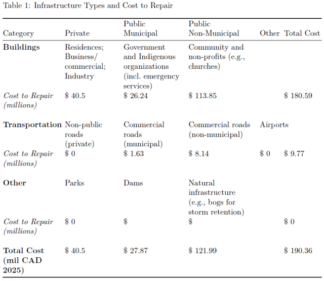
This figure shows the Infrastructure at Risk Table for a Coastal Flood for the Municipality of Carbonear.

The Summary of Infrastructure Damages (100-Year, No Action Scenario) section highlights the direct and indirect damages under 100-year return period with no preventative measures implemented. The figures show the direct and indirect damages in nominal dollars ($CAD 2025). These results provide insight into which asset types contribute most to total flood-related costs under baseline conditions.

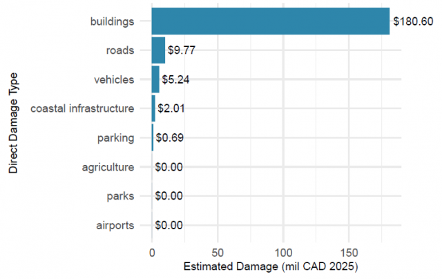
This figure shows the direct damages, which are the immediate physical losses caused by an event. They are related to the costs needed to fix or replace what was affected.

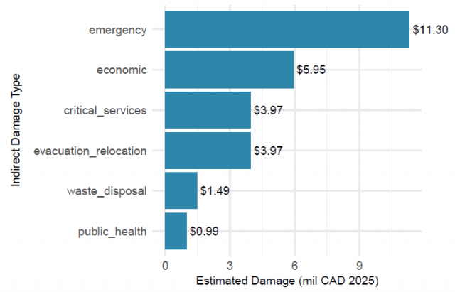
This figure shows the indirect damages, which are the secondary losses that occur because of an event, such as business interruptions or reduced access to services. They reflect the broader impacts that arise from the initial damage.

The Summary of Adaptation Strategies and Associated Costs outlines the range of potential prevention measures under consideration, along with the estimated capital and annual maintenance costs. Options selected in the CBATool_Inputs.xlsx file are addressed. Since No Action, Planned Retreat, and Protection were selected, these options will be included in the analysis.

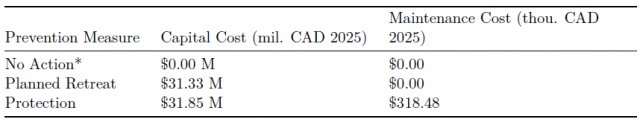
Options such as No Action, Planned Retreat, and Protection highlight the spectrum of responses available, from low-cost inaction to high-investment interventions.

The Summary of Cost Outputs summarizes the results of the economic cost-benefit analysis for a range of preventative measures. Preventative Measures shown in red represent options that are not economically beneficial based on the Benefit-Cost Ratio. Options shown in green are economically beneficial and worth undertaking. Options that are close to a neutral Benefit-Cost Ratio of 1.0 are left without highlighting.

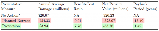
Each column in this figure provides a key performance metric used to evaluate the effectiveness and financial viability of flood adaptation strategies.

From the results in the Summary of Cost Outputs table, Protection would be recommended for further consideration for the municipality of Carbonear.

Scrolling down to the Preventative Measures section, new maps for each of the three primary preventative measures have been generated. Here, the user can visually compare how flood risks change under different management approaches, from taking no action to retreating from high-risk areas or protecting existing development.

The Damage Centres (100-Year, No Action Scenario) displays a heatmap that show areas with higher cumulative flood-relative damages across all infrastructure types under the 100-year No Action scenario. Areas with no or very low damages are masked out.

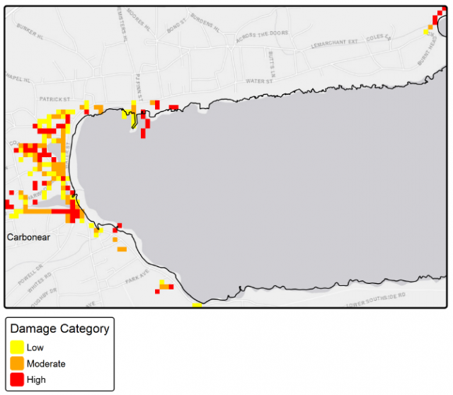
In this figure, brighter colours (red) indicate high damages, orange for moderate relative damages, and yellow for lower damages.

After reviewing the components of this report, the municipality of Carbonear should look further into considering Protection as a Preventative Measure for a Coastal 100-year flood.

5 Troubleshooting

For most issues, re-downloading the CBA Tool and starting anew will likely fix issues you are experiencing. Be sure to keep local copies well organized, and avoid modifying the files in the spatialdata, Rasters, and folders other than the output folder manually. The tools provided here will modify files in a way that is compliant with the tool.
If you experience an issue running the tool, you may need to contact your IT department to allow the CBATool.exe program to run. See section called ‘Security and File Permissions’.

5.1 Common Troubleshooting Tips

Here are some common questions or issues you may run into:

5.1.1 General Usage

Q: The CBA tool does not run and has an error that says something is “read-only”

A: You likely have a document from the outputs folder, such as the NLACBA_report or the cba_summary.xlsx open, which is preventing it from being overwritten when the CBA Tool is run again. Save and close the output files (keeping any you wish to keep in a separate folder or renaming them to something else), and then re-run the tool. This should overwrite or create new output files as long as the files are not open on your computer.

Q: How do I run the executable?

A: If you downloaded the zip file, unzip the file and go to the folder. Double click the Application called CBATool (it may appear as CBATool.exe). When you do this, it may open a window and run right away, or it may open a blue Windows Security windo that says, “Windows protected your PC”. If you see the option to click “More info” and then “Run anyway”, you can do that. If that does not work, you may need to contact your IT department to ensure that this executable can be run.

Q: I have an error that says that ‘Windows protected your PC’ when running the tool

A: You can enable the tool to run by clicking on More info and Run anyway. See screenshot below.

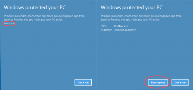
Q: I have an error that some data or .tif file is not available.

A: In the CBA_Inputs.xlsx tool, check that the correct preentative measure cells are selected in the Preventative Measures Selection section (rows 11-18). You can also confirm that each preventative measure has raster data in the /Raster folder for the selected municipality. This error may be caused by empty or missing data for that scenario, or creating new scenarios without adding the raster data for them.

Q: Does the tool run without an internet connection?

A: An internet connection is only required to download the tool. Once it is downloaded, you should not need an internet connection for any furhter use of the tool.

Q: How do I install a new version of the tool?

A: The tool does not need to be installed formally, you simply need to download the zip file for the new version of the tool and unzip it into a new folder. The old version of the tool can be deleted, though be sure to save any reports or Excel files you wish to keep.

Q: Will the tool overwrite the report from the last run?

A: Yes, the tool always writes reports to outputs/NLACBA_report.docx. If you wish to save that report and avoid having it be overwritten, you should move the files to another folder or rename the folder from outputs to something else.

Q: Can the tool be adapted for use with other hazards?

A: Yes – see section Section 3.4 for more information.

Q: Do I need Microsoft Excel or will open-source alternatives work?

A: Microsoft Excel is required, as the format for drop boxes does not appear to save properly in open-source equivalent software formats. However, this may be something that can be addressed in the future for those without Microsoft licensing.

5.1.2 Damages Calculations

Q: How does the tool use the flood depth to estimate damages for coastal infrastucture?

A: It does not, it uses data stored in the Coastal Damages sheet (hidden by default) to estimate damages based on wave height and water level. If you wish to modify this, you can use the Damage Modifiers tab to modify the damages with a multplier for specific assets, or edit the data in this sheet.

Q: I am getting zero damages, why?

A: It may be that your 20 year and 100 year rasters have zero values and/or do not intersect with any assets. Inspect these with the tools provided and confirm in the mapping that you have non-zero depths overlapping your buildings and roads.

Q: I see a warning about zero damages computed for a certain scenario

A: Same answer as above – there may be no assets within the raster, or the raster may have no depths in it. This occurs for some cases, such as a coastal raster generated for an inland community. Inspect these with the tools provided and confirm in the mapping that you have non-zero depths overlapping your buildings and roads.

Q: The coastal raster seems overly conservative, is it correct?

A: The coastal rasters were generated using a simplified bathtub model, and also assumes no mitigation from dams or other control structures. Both of these are more conservative assumptions. The simplified method of estimating nearshore waves may also lead to inaccuracies. Nonetheless, the rasters are a useful starting point for estimating coastal flooding impacts. If you feel the rasters are overly conservative, you may edit the No Action or any other raster using the Raster Editor tool.

Q: For coastal damages, how much should the flood be reduced behind an armourstone breakwater structure?

A: This depends a lot on the local conditions and the type of breakwater. However, some general rules of thumb: a large emergent (above the surface of the water) breakwater will provide more relief from storm surges than a submerged. An emergent breakwater may reduce significant wave height up to 90%, while a submerged breakwater may be reduction as low as 20%. The distance of the structure from the shore also controls how much impact the reduction has, and where that reduction may be felt. These numbers may be used to roughly guide the application of Damage Modifiers in the tool and editing in the Raster Editor.

5.1.3 Additional Apps (Raster Editor, Measure Tool, Spatial Data Viewer)

Q: The Raster Editor or Measure Tool launches with an empty map

A: It is possible that you have selected preventative measures that are not available for loading. You can try to close the browser, uncheck all preventative measures except for No Action, and try relaunching the tool with the Raster Editor or Measure Tool to see if the map now loads.

Q: Issue launching the Raster Editor, Measure Tool, Create Study Boundary tool, or one of the shiny apps

A: If you have an adblocker in place, it may prevent the window from appearing. You can try to disable the adblocker and see if that allows the app to run.

Q: In the Measure Tool, my depth shows -Inf

A: This will happen if the line or area is drawn completely out of the depth raster available. This is not an issue if you intend for the adaptation measure or structure to be outside of the current flood zone, otherwise redraw it overlapping the flooded area.

5.2 Contact our Team

This tool and supporting documentation has been developed by Heron Hydrologic for the Province of Newfoundland and Labrador. Heron is also continuing to provide support for data updates, bug fixes, documentation updates, and other technical support upon request.
For any questions or concerns regarding the technical approach or usage of the tool, please reach out to us at ECCInfo@gov.nl.ca.

5.3 Updates to the Tool

The tool is planned to be maintained under a maintenance agreement with Heron Hydrologic, and will be updated several times per year. The updates will be posted on the tool’s website as updated become available.

6 Glossary

Here are some common terms you may come across:

• No Action: baseline condition with no preventative measures applied
• Planned Retreat: establishes a 100-metre buffer from the coastline, with affected assets assumed to have zero retained value
• Protection: implementation of engineered or structural measures to defend against flooding
• Stabilization: shoreline reinforcement or land stabilization measures to reduce flood risk
• Abandonment: withdrawal from at-risk areas without replacement or protective intervention
• Accommodation: adjustments to buildings or land use (e.g., elevating structures, floodproofing) to reduce vulnerability while continuing occupancy
• Private: infrastructure owned and maintained by individuals, businesses, or private organizations (e.g., residential homes, commercial buildings)
• Public: infrastructure owned and maintained by government authorities (e.g., schools, hospitals, municipal buildings, emergency services)
• Public Non-Municipal: infrastructure owned and operated by non-municipal public entities, such as provincial or federal agencies (e.g., highways, utilities, and regional facilities)
• Direct Damages: immediate physical or structural damages to infrastructure and assets caused by flooding (e.g., building repairs, replacement costs)
• Indirect Damages: secondary or consequential impacts that occur as a result of flooding (e.g., business interruption, loss of services, or increased transportation costs)
• Coastal: considers damages and preventative measures related only to coastal flooding
• Coastal and Riverine: considers combined flooding impacts from both coastal and riverine (inland river system) sources
• Raster: a digital image/map made up of a grid of cells that represents a location, where each cell contains a specific value like elevation
• Cost-Benefit Tool: a tool that assesses the relation between the cost of implementing or not implementing a solution and the value of the resulting benefits
• Polygon: a straight-sided figure that can be drawn in the Measure Tool and Create Study Boundary Tool to capture an area or create a new raster
• Polyline: a straight line that can be drawn in the Measure Tool to capture a length
• Freeboard: a factor of safety added above the base flood depth. This is used in the Measure Tool